histogram

https://www.linkedin.com/pulse/histogram-hasnaa-hassan



Histogram




Hasnaa Hassan 

Hasnaa Hassan
Quality Assurance Manager at Delta Textile Egypt.
Published Mar 30, 2016
+ Follow
Description

–A frequency distribution shows how often each different value in a set of data occurs. A histogram is the most commonly used graph to show frequency distributions. It looks very much like a bar chart, but there are important differences between them. When to Use

–When the data are numerical.

–When you want to see the shape of the data’s distribution, especially when determining whether the output of a process is distributed approximately normally.

–When analyzing whether a process can meet the customer’s requirements.

–When analyzing what the output from a supplier’s process looks like.

–When seeing whether a process change has occurred from one time period to another.

–When determining whether the outputs of two or more processes are different.

–When you wish to communicate the distribution of data quickly and easily to others. Histogram construction

–Collect at least 50 consecutive data points from a process.

–Use the histogram worksheet to set up the histogram. It will help you determine the number of bars, the range of numbers that go into each bar and the labels for the bar edges. After calculating W in step 2 of the worksheet, use your judgment to adjust it to a convenient number. For example, you might decide to round 0.9 to an even 1.0. The value for W must not have more decimal places than the numbers you will be graphing.

–Draw x- and y-axes on graph paper. Mark and label the y-axis for counting data values. Mark and label the x-axis with the L values from the worksheet. The spaces between these numbers will be the bars of the histogram. Do not allow for spaces between bars.

–For each data point, mark off one count above the appropriate bar with an X or by shading that portion of the bar. Histogram Analysis

–Before drawing any conclusions from your histogram, satisfy yourself that the process was operating normally during the time period being studied. If any unusual events affected the process during the time period of the histogram, your analysis of the histogram shape probably cannot be generalized to all time periods.

–Analyze the meaning of your histogram’s shape. 

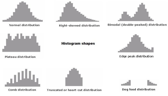
Normal

– A common pattern is the bell-shaped curve known as the “normal distribution.” In a normal distribution, points are as likely to occur on one side of the average as on the other. Be aware, however, that other distributions look similar to the normal distribution. Statistical calculations must be used to prove a normal distribution.

–Don’t let the name “normal” confuse you. The outputs of many processes—perhaps even a majority of them—do not form normal distributions , but that does not mean anything is wrong with those processes. For example, many processes have a natural limit on one side and will produce skewed distributions. This is normal — meaning typical — for those processes, even if the distribution isn’t called “normal”! 

Skewed

–The skewed distribution is asymmetrical because a natural limit prevents outcomes on one side. The distribution’s peak is off center toward the limit and a tail stretches away from it. For example, a distribution of analyses of a very pure product would be skewed, because the product cannot be more than 100 percent pure. Other examples of natural limits are holes that cannot be smaller than the diameter of the drill bit or call-handling times that cannot be less than zero. These distributions are called right- or left-skewed according to the direction of the tail. 

Double Peak or Bimodal

–The bimodal distribution looks like the back of a two-humped camel. The outcomes of two processes with different distributions are combined in one set of data. For example, a distribution of production data from a two-shift operation might be bimodal, if each shift produces a different distribution of results. Stratification often reveals this problem. 

Plateau

–The plateau might be called a “multimodal distribution.” Several processes with normal distributions are combined. Because there are many peaks close together, the top of the distribution resembles a plateau. 

Edge Peak

–The edge peak distribution looks like the normal distribution except that it has a large peak at one tail. Usually this is caused by faulty construction of the histogram, with data lumped together into a group labeled “greater than…” 

Truncated or heart-cut

–The truncated distribution looks like a normal distribution with the tails cut off. The supplier might be producing a normal distribution of material and then relying on inspection to separate what is within specification limits from what is out of spec. The resulting shipments to the customer from inside the specifications are the heart cut. 

Dog Food

–The dog food distribution is missing something—results near the average. If a customer receives this kind of distribution, someone else is receiving a heart cut, and the customer is left with the “dog food,” the odds and ends left over after the master’s meal. Even though what the customer receives is within specifications, the product falls into two clusters: one near the upper specification limit and one near the lower specification limit. This variation often causes problems in the customer’s process.